An agentic follow-up to a handwritten optimization of the von Mises–Fisher distribution.
I spent several days profiling, deriving, implementing, and testing a faster version of scipy.stats.vonmises_fisher.rvs. The first post tells that technical story: where SciPy spends its time, why the obvious shortcuts are dangerous, and how the handwritten Householder implementation came together.
This post asks the follow-up question. If coding agents receive the same SciPy source, a fixed ten-minute budget, and a strict verifier—but not my solution—how much of those several days of work can they recover?
The target is deliberately narrow: vonmises_fisher.rvs, which samples unit vectors concentrated around a direction mu, in dimensions from 2 to 2048. Each agent must return one faster solution.py. It receives a speed score only after passing interface and statistical checks. Reported timings use a full exclusive Slurm rerun on arton10.
The short version
- 13 of 24 valid agent submissions beat my 2.83× handwritten benchmark baseline; the best reached 11.41×.
- Most valid agent solutions reached roughly 2–5× geometric-mean speedup on the cluster.
- The common useful idea was algorithmic, not cosmetic: replace a dense rotation with an O(n·d) Householder transform or sample directly in the tangent space.
- The gain grew rapidly with dimension: leading solutions reached roughly 47–177× in the largest case.
- One high-effort submission was a clear outlier. It combined direct tangent-space construction with deterministic multithreading.
- Higher reasoning effort and API cost were not reliable predictors of performance.
- Fast but statistically wrong code received no valid score.
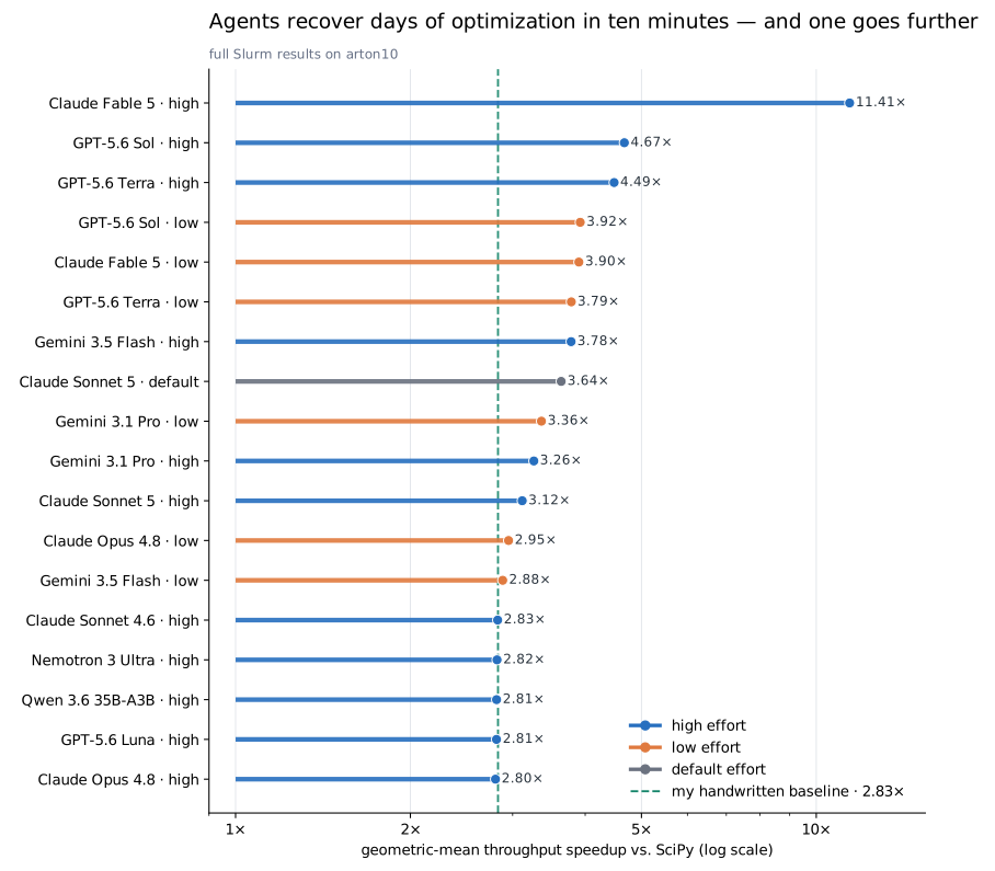
The several-day optimization behind the benchmark
The sampler first draws an axial component and a random tangent direction, then rotates samples from a canonical pole to the requested mean direction. The reference path uses a dense rotation whose cost becomes painful at high dimension.
| Stage | Reference-style cost | Optimized pattern |
|---|---|---|
| Draw axial coordinate | Wood rejection sampler | Keep the same exact distribution |
| Draw tangent direction | Gaussian vector + normalization | Vectorize and reuse output buffers |
Align with mu | Dense/QR-based rotation, effectively O(n·d²) | Householder reflection or direct tangent projection, O(n·d) |
| Large batches | Large temporary arrays | Chunking, in-place ufuncs, or controlled threading |
This was the key improvement in my handwritten work. The benchmark asks whether agents can recover it without seeing that implementation—and whether they can find anything beyond it—while preserving the probability law.
The publication controls were rerun under the same cluster setup. The SciPy wrapper measured 1.00×, while my handwritten NumPy Householder implementation reached 2.83× overall and 46.66× at dimension 2048. A deliberately wrong Gaussian sampler was faster at the largest dimension but failed the statistical gate.
| Control | Valid | Overall speedup | Speedup at d=2048 |
|---|---|---|---|
| SciPy wrapper | Pass | 1.00× | 1.00× |
| My NumPy Householder baseline | Pass | 2.83× | 46.66× |
| Wrong Gaussian | Fail | — | 53.01× |
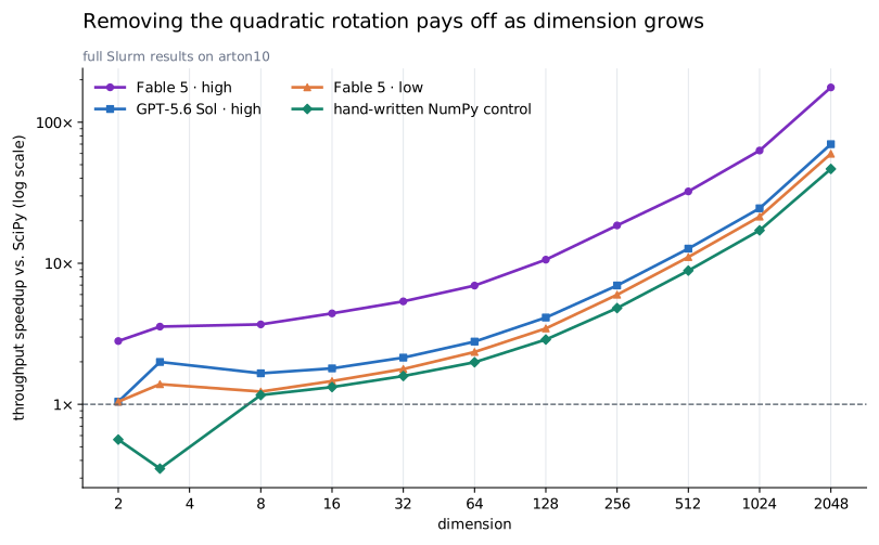
What the agents found
Many independently generated submissions converged on the same core design:
- Keep SciPy’s special cases in dimensions 2 and 3.
- Use Wood’s rejection sampler for the marginal cosine in higher dimensions.
- Generate a uniform tangent direction from normalized Gaussians.
- Replace the dense rotation with one Householder reflection.
- Reduce allocations with output buffers, in-place NumPy operations, and cache-sized chunks.
That convergence is the central result. The Householder route took me days of profiling, derivation, implementation work, and statistical testing. Many agents independently recovered the same asymptotic bottleneck and reconstructed the core algorithm in a ten-minute run. They were not merely tuning constants around the original implementation.
The outlier went one step further. Instead of constructing canonical samples and then rotating them, it projected Gaussian vectors directly into the tangent space of mu, scaled them by the sampled axial coordinate, and filled large batches across independent deterministic random streams. Because multithreaded speedups are sensitive to CPU topology, all reported results come from the same fixed-node cluster rerun with explicit thread limits.
Correctness is the gate, not a footnote
Sampling code can look plausible while returning the wrong distribution. The verifier checks:
| Check | What is tested |
|---|---|
| Interface | Shapes, float64 output, unit norms, seed determinism, stream advancement, invalid inputs |
| Distribution | Two-sample KS tests on projections onto mu and fixed random directions |
| Coverage | Dimensions 2–2048, several concentrations, and a rotation-sign edge case |
| Isolation | Only the submitted solution.py is imported in a fresh environment |
| Scoring | Geometric mean of throughput ratios, only if every correctness phase passes |
A deliberately wrong normalized-Gaussian control is very fast and still scores nothing. Correctness is a hard constraint, not a weighted objective that speed can compensate for.
Does more reasoning buy more speed?
Usually, only a little. In most paired runs, high and low effort landed on similar Householder implementations. The major exception was the high-effort outlier, which discovered a more aggressive parallel construction.
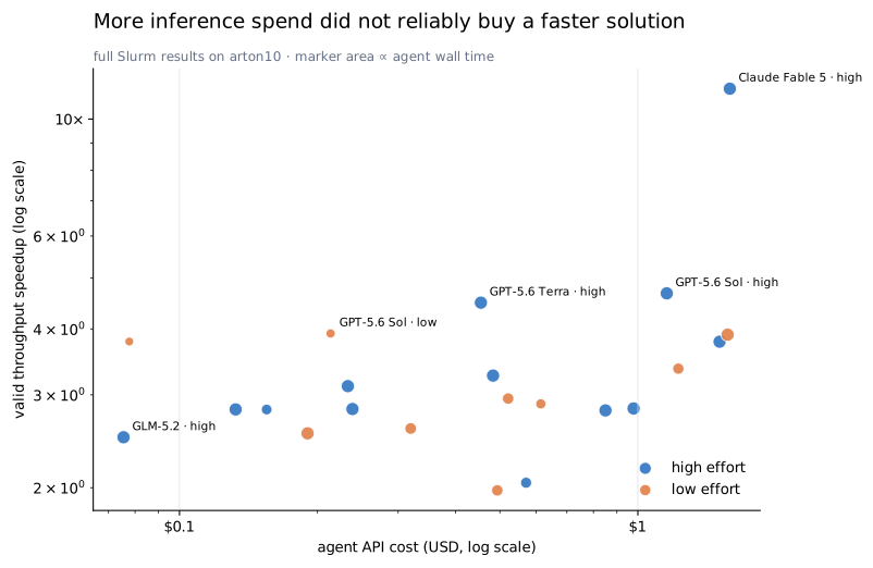
This is a small sample and not a model ranking in the general sense. It says something narrower: for this numerical task, once an agent recognizes the right algorithmic move, additional inference often changes implementation quality more than the core approach.
Benchmark protocol
The agent and verifier are separated. Agent runs may happen anywhere; final timing runs happen on one fixed CPU machine through Slurm.
prompt + pinned SciPy source
          │
          ▼
 coding agent (time/token budget)
          │  writes one solution.py
          ▼
 isolated correctness verifier
          │  pass only
          ▼
 fixed-node throughput + peak-RSS benchmark
          │
          ▼
 result JSON → tables and figures
For final measurements, submissions are synchronized to /itet-stor/aplesner/net_scratch, placed in a sequential Slurm job array, and run in the same Apptainer image on one exclusive arton CPU node. Each verifier is bound to four cores while the remaining cores stay idle. Math-library thread counts are pinned to those four cores.
| Reproducibility choice | Setting |
|---|---|
| Partition / node | cpu.normal / fixed arton10 |
| Scheduling | Slurm array, concurrency 1 |
| CPU allocation | Whole node exclusive; 4 bound cores per verifier |
| Environment | Python 3.12 Apptainer image with pinned NumPy and SciPy |
| Scoring | Geometric mean of throughput ratios across the RVS dimension grid |
The benchmark code, verifier, results, and reproduction workflow are available on GitHub. The publication manifest freezes the RVS-only scope, cluster jobs, source snapshot, and result hashes.
Limits and next checks
This is one routine, on one CPU architecture, with one scoring grid. Before treating the 11.41× outlier as a stable headline, I would repeat the finalists across independent allocations and separate one-core algorithmic gains from controlled four-core parallel gains.
- Repeat the finalists and handwritten controls to quantify between-run variation.
- Stress-test the leading solution across more seeds, concentrations, and near-pole directions.
- Rerun on a second CPU architecture.
- Compare speed at a fixed memory ceiling.
- Turn the simplest robust implementation into an upstream-quality SciPy patch.
The result here is narrow and, to me, surprising: under a strict statistical verifier, agents repeatedly recovered the bottleneck I had spent days working through, and several produced valid implementations faster than my baseline—not just faster wrong answers.