Faster von Mises–Fisher sampling with one reflection

Replacing a dense QR rotation with a single Householder reflection makes high-dimensional sampling dramatically cheaper.

Sampling from a von Mises–Fisher distribution has two parts: draw around the first coordinate axis, then map that axis onto the requested mean direction. The second step looks harmless, but constructing and applying a dense rotation becomes the dominant cost in high dimension.

What changed

The original SciPy implementation does two expensive things in its rotation path: it builds a dense orthogonal matrix with QR, then uses the general-purpose einsum contraction machinery to apply that matrix to every sample.

Original SciPy rotation pathsrc/vmf_scipy.py

embedded = np.concatenate([
    self.mu[None, :],
    np.zeros((self.dim - 1, self.dim), dtype=self.mu.dtype),
])
self.rotmatrix, _ = la.qr(np.transpose(embedded))

samples = np.einsum("ij,...j->...i", self.rotmatrix, samples) * self.rotsign

dense QR constructiongeneral tensor contraction

einsum is flexible, but it is not the best primitive for this repeated dense matrix–vector operation. A direct matrix multiplication expresses the workload more clearly and can dispatch to optimized linear-algebra kernels without the general contraction path.

Change 1 · keep QR

Use the vectorized NumPy path

The NumPy QR control keeps the same dense map, but uses numpy.linalg.qr and batched matmul. A substantial speedup is already available before changing the mathematics.

rotmatrix, _ = np.linalg.qr(embedded.T)
samples = (rotmatrix @ samples.T).T * rotsign

Change 2 · remove QR

Apply one Householder reflection

Because vMF is rotationally symmetric, we can drop the dense rotation entirely and store only the reflection vector u.

u = (e1 - mu) / np.linalg.norm(e1 - mu)
samples -= 2 * np.outer(samples @ u, u)

Why one reflection is enough

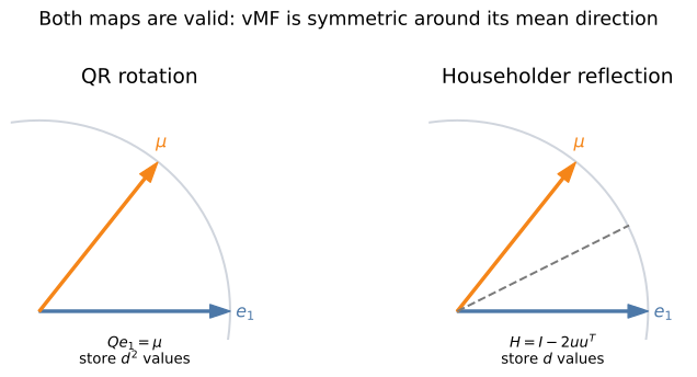
Comparison of a QR rotation and a Householder reflection mapping the first basis vector to the mean direction. — Any orthogonal map sending e₁ to μ is valid because vMF is rotationally symmetric around μ.

A single Householder reflection

H = I − 2uu^T, u = (e₁ − μ) / ‖e₁ − μ‖

maps e₁ to μ and preserves the distribution. It replaces a dense d × d matrix with one length-d vector and can be applied to a complete sample batch in place.

Implementations compared

The benchmark separates the array library from the orthogonal map. This gives QR and reflection implementations in both NumPy and PyTorch, alongside the original SciPy behaviour.

Reference baseline

SciPy QR

This path stays close to the original implementation: scipy.linalg.qr, batch rotation with numpy.einsum, and the legacy RandomState stream.

Same geometry, modern NumPy

NumPy QR

The dense QR map is unchanged, but the operations use numpy.linalg.qr, batched matmul, and a per-sampler Generator.

Proposed map

Householder reflection

The NumPy and PyTorch reflection variants remove QR. The in-place implementations reuse the sample output and avoid a second output-sized allocation.

Device-native sampling

PyTorch QR and reflection

The PyTorch paths keep batches row-major, normalize and scale owned tensors in place, and fuse the rank-one update with addmm. Samples stay on the selected CPU or GPU in float16, bfloat16, float32, or float64.

The measurements below use CPU float64 so all implementations can be compared directly. The PyTorch versions are included because practical workloads often need samples directly on an accelerator or in lower precision.

Throughput

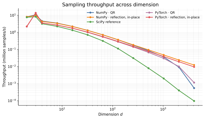
Dimension	NumPy QR	NumPy reflection	SciPy	PyTorch QR	PyTorch reflection
3	10.7 M/s	9.71 M/s	8.29 M/s	13.9 M/s	13.6 M/s
16	2.23 M/s	2.20 M/s	1.34 M/s	1.74 M/s	1.76 M/s
128	366 k/s	371 k/s	112 k/s	281 k/s	293 k/s
1024	36.5 k/s	47.8 k/s	2.00 k/s	30.2 k/s	38.5 k/s
4096	549/s	12.3 k/s	97/s	1.15 k/s	9.57 k/s

Speedup over SciPy

126.97×maximum measured NumPy speedup

99.01×maximum measured PyTorch speedup

End-to-end speedup of the in-place NumPy and PyTorch reflection implementations over SciPy. — End-to-end throughput ratios against the actual SciPy reference, not against the separate NumPy or PyTorch QR controls.

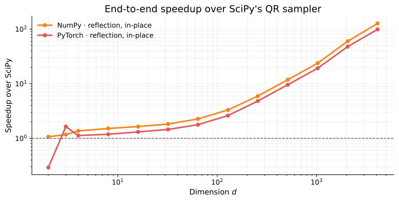
Implementation	Baseline	Geometric mean	Maximum measured
NumPy reflection, in-place	SciPy QR	6.28×	126.97×
PyTorch reflection, in-place	SciPy QR	5.01×	99.01×

The practical crossover is simple: random variate generation and dispatch dominate at tiny dimensions. As d grows, avoiding QR setup and dense matrix multiplication matters increasingly.

Complexity and random state

Area	Reflection path	QR reference
Map e₁ → μ	One Householder reflection	Dense QR rotation
Map construction	O(d)	O(d³)
Rotation storage	O(d)	O(d²)
Batch application	O(nd)	O(nd²)
NumPy RNG	Per-instance PCG64DXSM	Legacy RandomState in SciPy
PyTorch RNG	Per-device generator	Per-device generator

Benchmark details

CPU: AMD EPYC 7742
Workload: float64, κ = 50, dimensions 2–4096
Measurements: 273 raw timing rows

Timing: calibrated batches with a two-second window
Repetitions: three seeded runs
Allocation: 12 CPUs, one task at a time, no GPU

The implementation, raw measurements, and machine-readable tables are available on GitHub.

Appendix

Generalization to an older CPU

The headline benchmark uses the newer AMD EPYC 7742. To check whether the conclusion generalizes, the same CPU-only float64 sweep was repeated on an older Intel Xeon E5-2690 v2 with the same code, 12 allocated CPUs, and three seeds.

The older processor does not support AVX2, so PyTorch selects its generic CPU kernel path and is substantially slower there. These are hardware-generalization results rather than the primary performance numbers.

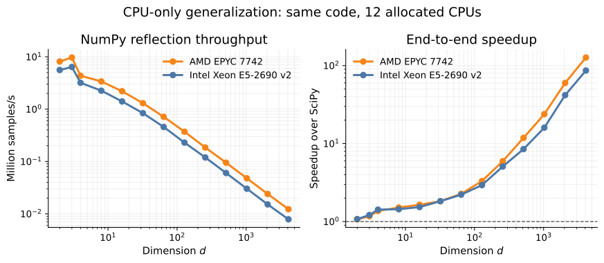
CPU-only generalization comparison between AMD EPYC 7742 and Intel Xeon E5-2690 v2.

Dimension	AMD reflection	AMD vs SciPy	Intel reflection	Intel vs SciPy
128	371 k/s	3.31×	230 k/s	2.93×
512	94.9 k/s	11.85×	60.3 k/s	8.50×
2048	24.0 k/s	59.86×	15.2 k/s	41.78×
4096	12.3 k/s	126.97×	7.86 k/s	86.45×

Full Intel Xeon E5-2690 v2 measurements

Throughput is reported as samples per second. Both speedup columns use the SciPy implementation on the same CPU as their baseline.

Dimension	SciPy QR	NumPy QR	NumPy reflection	NumPy vs SciPy	PyTorch QR	PyTorch reflection	PyTorch vs SciPy
2	5.21 M/s	5.61 M/s	5.60 M/s	1.08×	1.36 M/s	1.56 M/s	0.30×
3	5.27 M/s	7.43 M/s	6.40 M/s	1.21×	2.50 M/s	2.50 M/s	0.47×
4	2.24 M/s	3.30 M/s	3.19 M/s	1.42×	1.26 M/s	1.27 M/s	0.57×
8	1.57 M/s	2.33 M/s	2.26 M/s	1.44×	656 k/s	657 k/s	0.42×
16	915 k/s	1.45 M/s	1.41 M/s	1.54×	328 k/s	330 k/s	0.36×
32	460 k/s	864 k/s	840 k/s	1.82×	165 k/s	166 k/s	0.36×
64	206 k/s	442 k/s	457 k/s	2.21×	82.5 k/s	83.5 k/s	0.40×
128	78.4 k/s	218 k/s	230 k/s	2.93×	40.9 k/s	41.8 k/s	0.53×
256	23.5 k/s	100 k/s	120 k/s	5.08×	19.9 k/s	20.8 k/s	0.89×
512	7.09 k/s	39.7 k/s	60.3 k/s	8.50×	9.50 k/s	10.4 k/s	1.47×
1024	1.88 k/s	14.0 k/s	30.2 k/s	16.02×	4.26 k/s	5.21 k/s	2.77×
2048	363/s	3.85 k/s	15.2 k/s	41.78×	1.67 k/s	2.57 k/s	7.08×
4096	91/s	712/s	7.86 k/s	86.45×	526/s	1.26 k/s	13.86×